Polynomial Functions

Numeric Representation

x g(x) 0 –250 10 0 20 50 30 –100

x h(x) 0 0 2 36 7 –14 10 100

Polynomial trends in a data set are recognized by the maxima, minima, and roots – the "wiggles" – that are characteristic of this family. Describing such trends with an appropriate polynomial is complicated by the fact that there are so many possible parameters: The degree of a polynomial, and the number of adjustable coefficients, can be as large as we want.

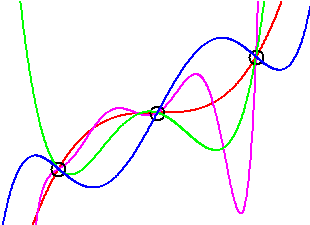
In general, given any data set, we can find a polynomial that describes every single input-output pair – exactly. In fact, we can find many such polynomials, of higher and higher degree:

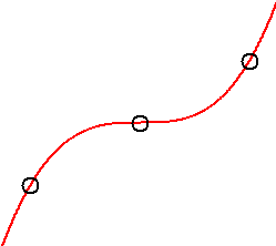
We typically choose the polynomial of least degree – the simplest model – to describe a data set:

It is natural, of course, to question whether or not we want a polynomial model to pass through every single data point. Statistical fluctuations and experimental error usually produce variations in data that are not representative of overall trends. Slavishly following every idiosyncrasy in a data set may not produce an accurate description of the big picture. Moreover, polynomials of high degree (necessary for many max and min) may be difficult to work with.

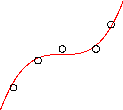
The alternative is to find a simple polynomial of low degree that follows the general trend in the data. Such a polynomial may pass above or below many of the data points, but still accurately describe the data as a whole:

This is the method of parametric curve fitting.

The decision about which route to take – exact fit or general fit – usually depends on two crucial factors: the number of data points and your confidence in the accuracy of those data points. The higher your confidence in the data, the more likely it is that you will want a polynomial to follow all of its ups and downs. Confidence decisions will depend on the provenance of the data set. They may also depend on a statistical analysis of the variations within the data – a subject for a course in statistics.

A polynomial that passes through every single data point is usually called an interpolation polynomial. The general method for finding interpolation polynomials is described in the hint below.

Lagrange interpolation polynomials:

For large data sets, low degree interpolation polynomials called splines are sometimes used to describe small groups of adjacent data points, and then connected together into a description of the entire data set. An outline of such a method, using cubic splines, is described in the hint below.

Cubic splines:

A polynomial that follows only the general trend in a data set, perhaps passing above some of the data points and below some of the others, is usually called a regression polynomial. A quick cataloguing of a data set's ups and downs is often sufficient to produce a regression polynomial of low degree.

For example, consider the data for  g  above:

x	g(x)
0	–250
10	0
20	50
30	–100

We observe that the data quickly rises between  x = 0  and  x = 10 , crosses the x-axis at  x = 10 , peaks somewhere between  x = 10  and  x = 30 , and then dives down, crossing back over the x-axis between  x = 20  and  x = 30 . This is enough information to find a reasonable polynomial.

The polynomial of lowest degree with a single peak is quadratic. We know there is a root at  x = 10 , and we might estimate the second root at, say,  x = 25 . This gives a general form of  g(x) = a (x – 10) (x – 25) = a x ² – 35 a x + 250 , where  a  is an adjustable parameter. A plot of the data and the equation together, and some experimentation with various values for  a , shows that  a = –1  and  g(x) = – x ² + 35 x + 250  provide a reasonable (in fact, an exact) fit:

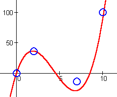
Similarly, consider the data for  h  above:

x	h(x)
0	0
2	36
7	–14
10	100

There are at least three roots: One at  x = 0 , one between  x = 2  and  x = 7 , and one between  x = 7  and  x = 10 . If we arbitrarily pick the midpoints of the intervals on which the latter two roots lie as our approximations of them, then we are led to a general form of  h(x) = b (x – 0) (x – 4.5) (x – 8.5) = b x ³ – 13 b x ² + (38.25) b x , where  b  is an adjustable parameter. Again, a plot of the data and the equation together, and some experimentation with various values for  b , shows that  b = 1.1  and  h(x) = (1.1) x ³ – (14.3) x ² + (42.075) x  provide a reasonable fit:

Adjusting the approximations of the roots left and right (and then  b  again) might produce even better results.

You might wonder which polynomial produces the best fit to a data set. The answer, of course, depends on the meaning of "best". If "best" means "exact", then the answer is an interpolation polynomial. If "best" means "best regression polynomial" of a certain degree, then the answer is more subtle. We must make an accounting of the errors a polynomial makes each time it misses a data point, and sum up these errors over the entire data set. There is a systematic method for making this sum of errors as small as possible, and so, indeed, for finding the "best" regression polynomial of a certain degree. It is called the method of least squares, and it is used by most computer programs when fitting curves to data. The method is outlined in the hint below.

The Method of Least Squares: