Logistic Functions

Numeric Representation

x g(x) –30 0.14 –20 0.36 –10 0.88 0 2.00 10 3.93 20 6.27 30 8.14 40 9.19 50 9.67 60 9.87 70 9.95

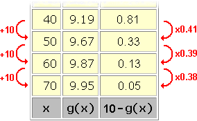
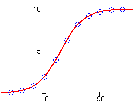
A quick inspection of the output values in the data table for  g  at right shows the typical pattern for logistic growth: Small initial rates which then accelerate up to a point of inflection, after which the growth slows down and eventually approaches a limiting value. We are fortunate to have a data set which displays the entire progress of a logistic function's S-shaped growth, and so makes the choice of a logistic model a natural one. Often, however, we may have data on only a small part of this curve – parts which, in isolation, may be indistinguishable from forms of exponential growth. For example, exponential growth displays a pattern of increase by constant multiples over equal input intervals. (See the section on numeric representations of exponential functions.) The early parts of the data for  g  show approximately this pattern:

In the early stages of logistic growth  f(x) = a / (1 + b c ^–x) , c > 1 , the outputs are rather small. This is because the exponential in the denominator is rather large. In particular, it is much larger than  1 , and adding the  1 + ...  in the denominator has little affect on the output. Thus, for small outputs, logistic growth behaves approximately like the function  y = a / (b c ^–x) = (a / b) c ^x .

Likewise, the latter part of logistic growth can be difficult to distinguish from bounded exponential growth. Near its limiting value, logistic growth  f(x) = a / (1 + b c ^–x)  behaves approximately like the function  y = a (1 – b c ^–x) . That is, like a function for which  a – y  is an exponential  (a b c ^–x).

If we use  a = 10  as our limiting value (the data seems to be approaching it) and look at  a – g(x)  in the latter stages of the data's growth, we once again see an approximation of exponential growth:

We use the similarities between logistic growth and exponential growth to find suitable values for the parameters  a , b , and  c  in a logistic model  f(x) = a / (1 + b c ^–x)  for a data set.

The parameter  a , as we have noted, is just the data's limiting value. Unless the data displays the latter stages of logistic growth, and the limiting value is quite obvious (approximately  10  in the data set for  g), it may take some trial and error to find a value for this parameter that will fit the data.

Values for the parameters  b  and  c  are found using properties of exponential functions.

In the early stages of growth, when the model behaves approximately like  y = (a / b) c ^x , each input interval from  x  to  x + Dx  results in an approximate ratio of outputs:

In the data set for  g , Dx  = 10  and this ratio is approximately  2.4 . Thus, c = (2.4) ^1/10 = 1.1 .

Similarly, in the later stages of growth, when  a – y  behaves approximately like  a b c ^–x , ratios for  a – y  are:

In the data set for  g , Dx  = 10  and this ratio is approximately  0.4 . Thus, c = (0.4) ^–1/10 = 1.1 , as we found before. The agreement at either end of the data set is a reassuring sign that the logistic model is appropriate here.

Having found a and c, we can usually adjust  b  until the model fits the data. In this case, a value of  b = 4  works well: